Analyzing Google Trends with Matrix Profile
Recently, I've been reading about the matrix profile. It is a recent algorithmic discovery in time-series analysis, allowing for efficient "time series motif discovery, time series joins, shapelet discovery (classification), density estimation,... etc.". There is a wealth of papers, videos, and applications for the algorithm on the project's webpage. The most interesting aspect of the matrix profile, at least to me, were its applications to motif discovery and conversely anomaly detection.
Simply put, anomaly detection is the identification of spurious or rare events. A good anomaly detection algorithm should make it clear when such an event occurs, with few false negatives or false positives. I started off by downloading an R implementation called tsmp, and applying the matrix profile to the temperature and particulate matter (PM) data from my home. However, the results were disappointing. I believe that this is due to the fact that most events for a temperature or PM change in my home were random or had no pattern.
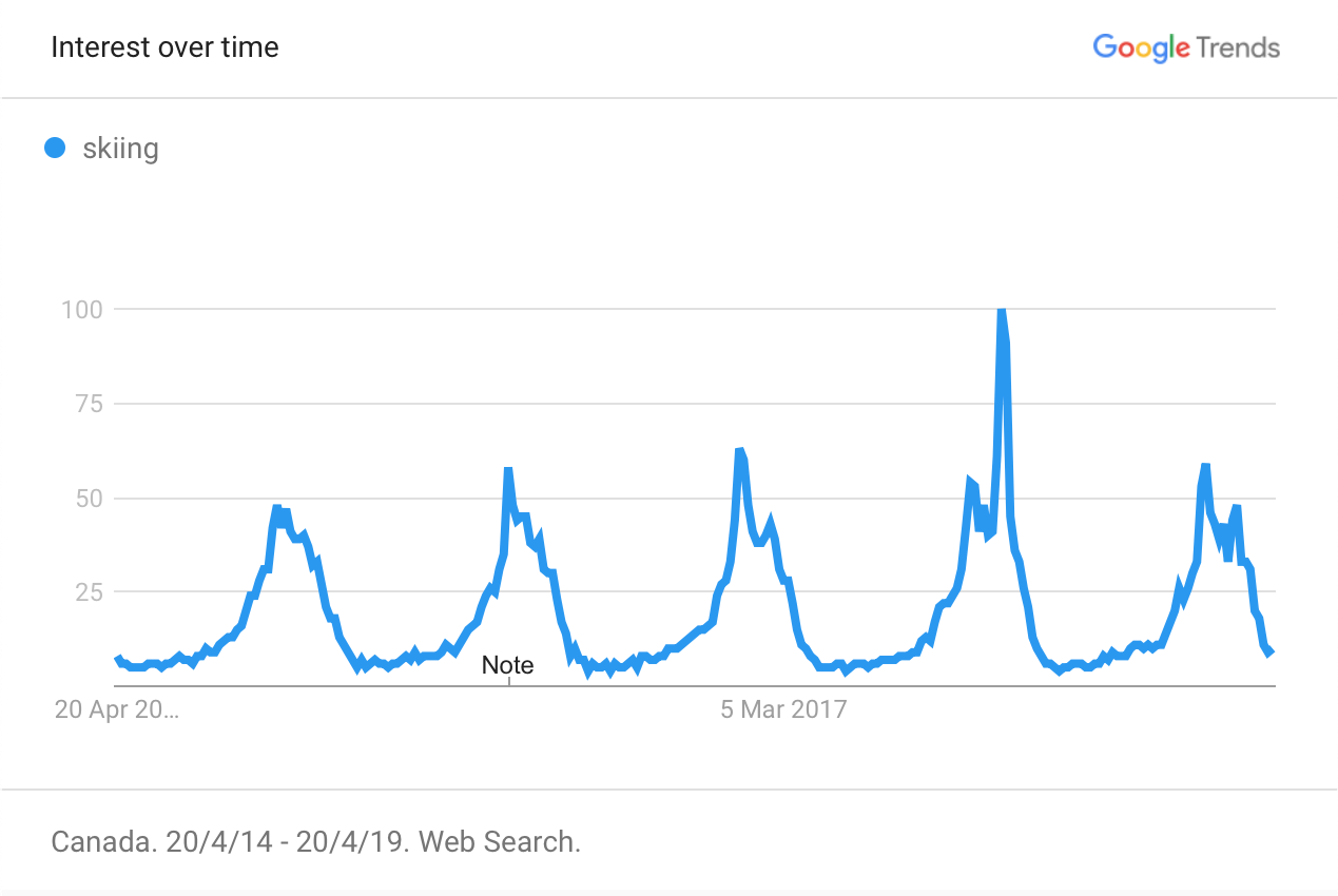
However, since aggregated data tends to show less noise, I thought of using search patterns from Google Trends. I downloaded the gtrendsR package and followed this guide on using the query functions. I decided to use the trends for the search term "skiing", which showed a sharp increase during the 2018 Winter Olympics.
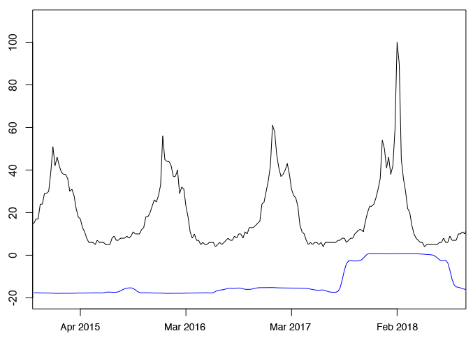
The following is a plot of the matrix profile against the time-series data: high values indicate new or unseen motifs, while low values indicate motifs that have already been seen nearby. You can see the matrix profile has picked up the sudden change in searches during the beginning of 2018.
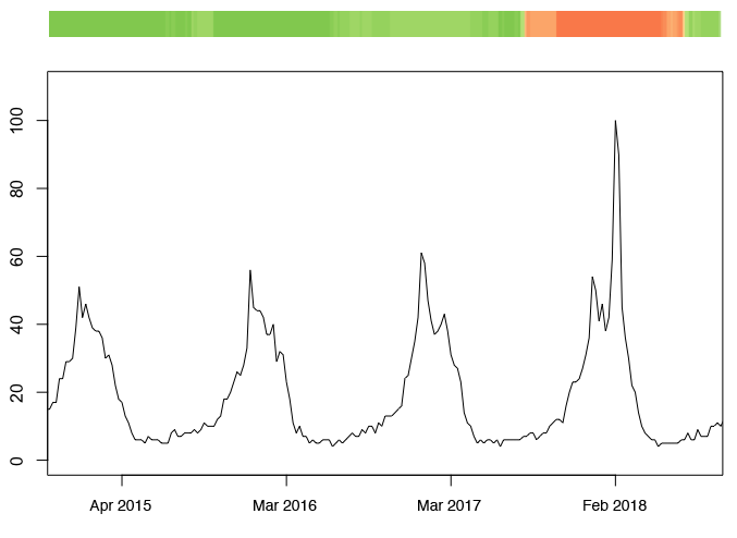
Finally, I thought that visualizing the matrix profile through a colour gradient would be more intuitive. The following is a plot with a heatmap above the original data. Personally, I think this looks better and is quicker to understand.
R Code for Matrix Profile and Graphs
library(tsmp)
library(smoother)
library(gtrendsR)
library(reshape2)

# Get Google Trends for skiing
google.trends = gtrends(c("skiing"), geo = c("CA"), gprop = "web", time = "today+5-y")[[1]]
google.trends = dcast(google.trends, date ~ keyword + geo, value.var = "hits")
rownames(google.trends) = google.trends$date
google.trends$date = NULL

# Generate Matrix Profile
matrix <- stomp_par(google.trends$`skiing_CA`, window_size = 50, n_workers = 4)

# Some Gaussian Smoothing over the Matrix Profile
smp <- smth(matrix$mp, window = 0.03, method = "gaussian")

# Squish margins
par(mai = c(0.42, 0.82, 0.22, 0.22))
plot(google.trends$`skiing_CA`, type = 'l', xlim = c(35, 225), ylim = c(-20, 110))
lines(25:(length(matrix$mp) + 24), smp * 7 - 26, type = 'l', col = "blue")

# Generate the 1-column Heatmap
library(RColorBrewer)
coul = colorRampPalette(brewer.pal(2, "RdYlGn"))(24)
heatmap(cbind(-matrix$mp, -matrix$mp), col = coul, Colv = NA, Rowv = NA, scale = "column", labRow = NA, labCol = NA)